[…] This article is the second of a three-articles series. Read the first part here: Partition Tables – Ways to Improve Performance in your SQL Server Environment. This article is focused on implementing the techniques from in the first article, and checking the […]
Note: This article is the first of a three-article series. I hope the sequence will help you to improve the performance in your systems using Partition Table and ColumnStore Index.
The set of articles is focused in introduce you to Partition Tables statements and a benefits to use these techniques in a scenario where you should write in a table with ColumnStore Index. Remember, in SQL Server 2012 the ColumnStore Index change the table to read-only, and this kind of index was launched in SQL Server 2012, but you can use the Partition Table since SQL Server 2005. In this first article, let’s understand the benefits and terms to why to use the Partition Table, the second one will show how to implements the Partition Table and check the improvement in logical reads, and the third we will see how to create the ColumnStore Index in a table and how to write there. Keeping in the third, let’s compare techniques and process expended in each way to done this task.
First of all, let’s create a database to use in our samples. I didn’t used the AdventureWorks because it’s a fully configured and working model, and I know it’s not the real environment that most of customers that we visit and work for. Then, let’s create a database to store information about visitants in a building. For these articles, think of a hypothetical museum that open the door the first time in Jan/2013 and works hard during all 2013. During this period, there are around 10 million visits. To show this demonstration, let’s split the visitors per months writing each month in each partition. In the first step, let’s create the table and insert all the rows inside together.
CREATE DATABASE dbMuseum
GO

USE dbMuseum
GO

CREATE TABLE tbVisitors
(id INT IDENTITY(1,1) PRIMARY KEY
,name VARCHAR(50)
,date DATE)
GO

INSERT INTO tbVisitors(name, date)
VALUES (newid(),
convert(date, convert(varchar(15),'2013-' +
convert(varchar(5),(convert(int,rand()*12))+1) + '-' +
convert(varchar(5),(convert(int,rand()*27))+1))))
GO 10000000
After some minutes, there is a table with 10KK random rows in dates between Jan & Dec/2013. Now, let’s understand what Partition Table is.
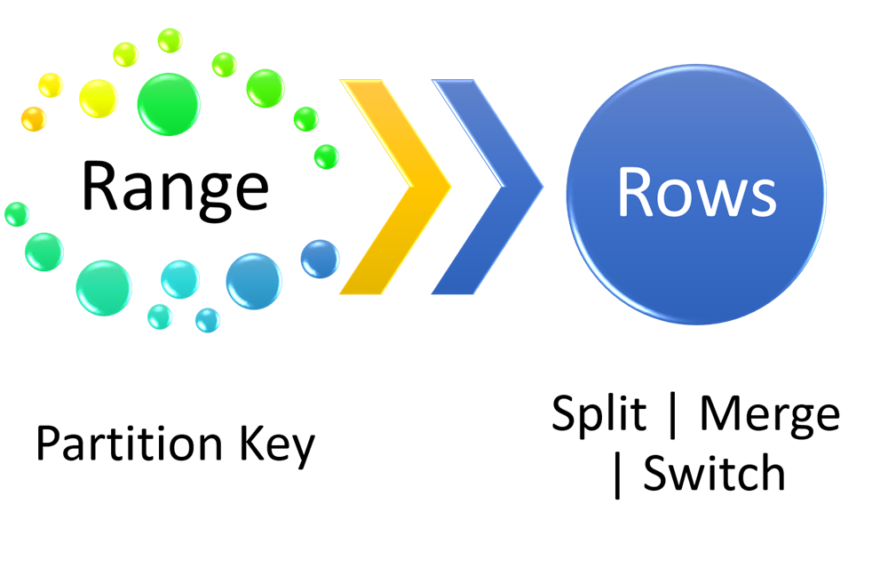
Basically, the Partition Table is divided in four steps. Starting storing the rows in tables and indexes, if don’t define a specific File Group, those rows are stored in default file group. However it’s possible to create a table or index informing the Partition Scheme that will store in a defined File Group. Each Partition Scheme could be mapped in one or more File Groups. The rows are direction to right File Group based in algorithm created in the Partition Function. The flow is something like this:
Partition Table is a technique used in data architecture to improve performance and management of data, splitting the rows in different tables and (if wants) File Groups, based in a parameter. Some people ask why partitioning? Think of a single table storing all the records about some entity, like sales or access. I know, normally we design the table to store this rows without any problem, but it’s not the regular scenario for the companies, I have already seen some VLDB (very large databases) with no index in tables used to reports, and these reports spent more than three hours just to tell the sales amount for last month. It’s sad, but it’s possible to find in some customers!
Obviously, neither all VLDBs should be improved with Partition Table, all of us know this, but split the “historical” data and “actual” ones should getting better the request velocity. When we talk about Partition Table, it’s good to pay attention to scalability and maintenance of data; using these techniques we improve, even these topics, also the disk. Think about a storage that we can manage the disks, storing the “historical” data in a poor disc IDE 5400RPM than the “actual” ones stored in a SAS 15K. Remember that report some lines up? Alignment both data and indexing partition, the request just read pages in the rich disk and the times goes from three hours to just some milliseconds.
One other application to Partition Table, is to use data from the last three years to forecast the next one. If you request the summarization in a single table, you could be your competitor, blocking the table and causing a wait for the real customer in your solution. It’s not good to an e-commerce in the Christmas holiday times, right?
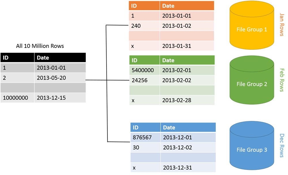
For example, look at the image bellow. All the 10 million rows are stored in the same table (tbVisitors) in the first moment (Black left table). After the partition, using the month as parameter, one table store rows only for that month (Orange for January, Green for February, Blue for December), creating 12 tables (in the same File Group, or not).

To apply the Month parameter it’s necessary to define the range that the algorithm (Partition Function, remember?) will use to split the rows. This range works together the Partition Key, which is a unique key value used to be logical data splitter. After the data stored in separated partitions, its possible use some functions to move and/or manage data from a partition to another one. Using Merge statement its possible join rows from two partitions to just one, in other hand is possible to use the Split statement to divide one single partition in two partitions. Another statement is Switch, used to move the partition set as “actual” to “historical” or vice-versa.

Looking at the example above, the rows are split based in month, the column Date is used as Partition Key, and the Range will start in the first day each month and finish in the last day for that month. Something like this:
Range 1, starting Jan/1st and finish Jan/31st
Range 2, starting Feb/1st and finish Feb/28th
…
Range 12, starting Dec/1st and finish Dec/31st
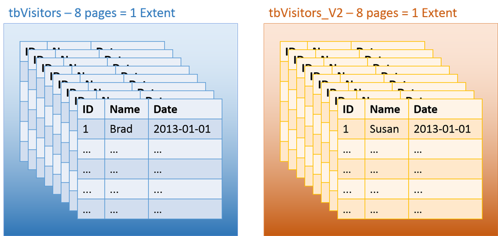
Even the Filegroup being the last step in the process, it is possible go back and create the Partition Function and Partition Scheme in the environment. Just to remember, all data are stored in 8Kb pages, and a set of 8 pages (64 Kb) are called Extent. Independent the page store just one register, SQL Server will create and allocate 8Kb for that page. Another thing is, one page should store data from just one table; it’s impossible store rows from more than one table. Thinking of the example, even if we add just one row at the table tbVisitors, SQL Server will allocate 64Kb in the disk. If we created another table, and stored only one row there, another extent will be created and allocate another 64Kb in the disk, even if there is enough space in the first extent. It happens after the first extent been used, because the first one will be shared between the objects, after the first 64Kb stored, each table create own extent. Look at the example below.

Knowing this storage structure is important, because the process for indexing and requesting information from the database is measured based in quantity of Logical Reads that the SQL uses to return the information. The more pages read, the more expensive the query!
The second article in this series will cover creating all steps about the Partition Table, and checking the Logical Reads.

That is a good article but… there are so many language mistakes in the text that at some point it makes it really hard to read. Could you please re-check the text and correct the mistakes? Thanks a lot.